Maximum Likelihood Estimation of Network Size by N Parallel k-lookups in Kademlia DHT

PDF version 🔗

1. Introduction

The lookup (often informally referred to as "k-lookup") is the primary and most crucial function in the Kademlia peer-to-peer distributed hash table (DHT) protocol [1]. It is a recursive, iterative algorithm designed to locate the $k$ closest nodes to a specific target ID within the network. The final set of $k$ closest nodes found has XOR distances that are minimised within the network, and the magnitude of these distances is related to the density of nodes, which itself depends on network size $n$. It's clear that performing several lookups to random $N$ target nodes, we get more information about anticipated network size. A method of estimation $n$ by processing $N$ parallel k-lookups is proposed in [2]. It's based on the fact that distances in each ordered set of k-lookup are the order statistics with specific beta distributions which depend on $n$. Then, according to the method of moments (MoM) [3] the estimator for $n$ is obtained by matching the expected value of the beta distribution with the empirical result by averaging distances from lookup data. The suggested estimator is great from a practical point; however, some aspects of the provided solution are heuristic, e.g., the ways of averaging sample data. It's also hard to make assumptions on the efficiency of the MoM estimator, because there is no way of getting theoretical minimum variance for any unbiased estimator.

Using the same model as in [2], the current work considers Maximum Likelihood Estimation (MLE) [4]. The MLE is generally preferred over MoM because it produces more efficient, consistent, and often unbiased estimators with stronger theoretical properties. MLE requires no heuristic assumption and can be derived directly from the joint Probability Distribution Function (PDF) of distances from N parallel k-lookups. The joint PDF also allows us to get the Cramér-Rao bound [5] for minimal variance of the efficient estimator.

The main results of the work are:

• the MLE estimator (3), which uses the average of logarithms of normalised distances from $N$ random $k$-lookups;
• the Cramér–Rao bound (4) for minimal variance of the efficient estimator and its approximations (6-7);
• illustration of the efficiency of the MLE estimator by results of computer simulation.

2. The model

Kademlia distance estimation works by querying $k$ "closest" nodes to a random target ID.

Let $D_1, \dots, D_n$ be XOR distances from a probe node to all $n$ network nodes, and $U_i = D_i/(2^L-1)$ are normalised distances for $L$-bit addresses. $U_1, \dots, U_n$ are modelled as independent random variables uniformly distributed on $(0, 1)$.

The result of a single lookup is the ordered set of $k$ smallest distances $\{U_{(1)}, \dots, U_{(k)}\}$ selected from $U_1, \dots, U_n$. Here $U_{(i)}$ is the distance to the $i$-th closest node. So, we observe the first $k$ order statistics [6] from a sample of normalised distances $U_1, \dots, U_n$.

When performing several k-lookups to N random probes, we make an assumption that all N samples of distances (so, the observed order statistics) are independent.

3. The likelihood function

For a single lookup the likelihood function (LF) is the joint PDF of the first $k$ order statistics $U_{(1)}, \dots, U_{(k)}$ from a sample of size $n$:

$$\begin{gather*} f_{U_{(1)}, \dots, U_{(k)}}(u_1, \dots, u_k \mid n) = \frac{n!}{(n-k)!} (1 - u_k)^{n-k}, \\ \text{for} \quad 0 < u_1 < \dots < u_k < 1 \tag{1} \end{gather*}$$

We derive this later, but notice an important fact now: the optimal ML estimate of $n$ can be obtained by taking into account only $k$-th order statistics. The statistics up to $k$ are irrelevant to the estimate. In other words, to estimate the network size, only the last k-th distance in ordered lookup results is sufficient.

This conclusion can be generalised for the optimal Bayesian estimator, because the LF as a part of the posterior distribution is the only place which captures the observation.

Note that the heuristic solutions proposed in [2] take into account all distances from the lookup result.

Using simplified notation, true in the area where LF differs from zero

$$f_1(u \mid n) = \frac{n!}{(n-k)!} (1 - u)^{n-k}$$

and taking into account the assumption on independence of the samples, we get the LF for several k-lookups to N random nodes:

$$\begin{align*} L(n) &= \prod_{i=1}^{N} f_1(u_i \mid n) = \\ &= \left[ \frac{n!}{(n-k)!} \right]^N \prod_{i=1}^{N} (1 - u_i)^{n-k}, \tag{2} \end{align*}$$

where the observation $u_i$ is the $k$-th smallest normalised distance taken from the $i$-th lookup.

4. Maximum likelihood estimate

The MLE estimator $\hat n$ maximises (2). It means that $\hat n$ is an integer at which the likelihood sequence $L(n)$ stops increasing and starts decreasing. To find it, consider the ratio function $G(n) = L(n) / L(n - 1)$ and the conditions the $\hat n$ conforms to:

1. The likelihood is increasing up to $\hat n$: $G(\hat n) \ge 1$.
2. The likelihood starts decreasing after $\hat n$: $G(\hat n + 1) < 1$.

As follows from (2), the ratio function is:

$$G(n) = \left( \frac{n}{n-k} \right)^N \prod_{i=1}^{N} (1 - u_i)$$

and within rounding error the MLE is the root of equation $G(n) = 1$:

$$\hat n = \frac {k} {1 - \left[ \prod_{i=1}^{N} (1 - u_i) \right]^{1/N}}$$

From a practical point of view, the last expression is easier to implement in the equivalent logarithmic form:

$$\begin{align*} \hat n &=\frac{k}{1 - \exp(\overline{L}_u)}, \\ \text{where} \quad \overline{L}_u &= \frac {1} {N} \sum_{i=1}^{N} \ln(1 - u_i) \tag{3} \end{align*}$$

Algorithmically, the estimator (3) performs the following steps:

1. For each lookup $i \in \{1, \dots, N$}, which consists of $k$ smallest distances to random targets:
   • select the maximal distance $d_i$;
   • calculate logarithmic metric $\ln(1-u_i)$ for the normalised distance $u_i = d_i/(2^L-1)$.
2. Calculate average $\overline{L}_u$ on the $N$ metrics.
3. Estimate the network size.

As expected, the estimator (3) always produces a result greater than $k$, because $\overline{L}_u$ is negative. The two edge cases when $u_i\text{s}$ are nearing to $0$ ($\hat n \to \infty$) or to $1$ ($\hat n \to k$) are also intuitively understandable.

5. Efficiency of the estimate

MLEs are known for their strong theoretical properties. For large sample sizes, they are consistent (converge to the true parameter), asymptotically normal, and asymptotically efficient (achieve the lowest possible variance).

Treating $n$ as a continuous parameter, the variance of the efficient estimator [5] is given by Cramér–Rao Lower Bound (CRLB):

$$\text{Var}(\hat{n}) \ge \frac{1}{I(n)}$$

where the Fisher Information is obtained by averaging of the second derivative of the log-likelihood (2):

$$I(n) = - E \left[ \frac{\partial^2}{\partial n^2} \ln L(n) \right]$$

The log-likelihood for N observations is:

$$\begin{align*} \ln L(n) = N \cdot \ln \frac {\Gamma(n+1)} {\Gamma(n-k+1)} + \\ + (n-k) \sum_{i=1}^{N} \ln (1 - u_i), \end{align*}$$

where $\Gamma(x)$ is the gamma function. Differentiating this two times, obtain:

$$I(n) = - N \left[\psi'(n+1) - \psi'(n-k+1) \right]$$

where $\psi'(x) = \frac{\partial^2}{\partial x^2} \ln \Gamma(x)$ is the trigamma function [7].

So, the result for minimal variance is:

$$\begin{align*} \text{Var}(\hat{n})_{min} &= \frac{1}{I(n)} = \\ &= \frac{1}{N \left[ \psi'(n-k+1) - \psi'(n+1) \right]} \end{align*} \tag {4}$$

Next, the difference of trigamma functions in (4) we approximate with:

$$\psi'(n-k+1) - \psi'(n+1) \approx \frac {1} {n-k} - \frac {1} {n} \tag {5}$$

The approximation (5) is quite good, especially when $n$ is large and $k$ is small relative to $n$. Indeed, we get (5) using a known series representation [7] and substituting the sum by an integral:

$$\begin{align*} \psi'(n - k + 1) - \psi'(n + 1) = \\ = \sum_{j=n-k+1}^{n} \frac{1}{j^2} \approx \int_{n-k}^{n} \frac{1}{x^2} \, dx \end{align*}$$

Finally, in practice it is often convenient to normalise estimation error to the estimated value. Substituting (5) into (4) and dividing the result by $n^2$, we obtain an expression for normalised variance, which defines the potential precision of the MLE estimator:

$$\begin{align*} \sigma^2_{min} &= \text{Var}\left(\frac{\hat{n}}{n}\right)_{\min} \approx \frac{1}{N} \left( \frac{1}{k} - \frac{1}{n} \right), \\ &\text{where} \quad n > k \tag {6} \end{align*}$$

It is worth noting that in practice when network size $n$ is much larger than $k$ the normalised variance of efficient MLE is mainly determined by the values of $N$ and $k$, rather than $n$. For example, having $k=8$ and $N=10$, the standard deviation $\sigma_{min}$ increases only from 10% to 11%, as network size grows from 50 to $10^6$ nodes. Without the dependence on $1/n$ in (6), the standard deviation of the MLE estimator can be calculated as

$$\lim_{n\to\infty} \sigma_{min} = \max_{n} \sigma_{min} = \frac{1}{\sqrt {N k}} \tag {7}$$

6. Results of statistical simulation

The simulation [8] was performed to compare the precision of the MLE estimator (3) with the theoretical lower bound (6). We process 10,000 estimations for each combination of parameters $k = {8, 20}, N = {10, 20, 40}$ and network sizes $n = {25, 10^2, 10^3, 10^4, 10^5}$. Each estimation receives $N$ statistics of $k$-th order from $n$ independent random variables uniformly distributed on $(0, 1)$. The normalised errors are then used to calculate the sample variance $\sigma^2$ which is the subject of comparison with the theoretical lower bound $\sigma_{min}^2$ (6).

$(N,\ k)$	$n=25$	$n=10^2$	$n=10^3$	$n=10^4$	$n=10^5$
$(10,\ 8)$	$0.09724$	$0.11158$	$0.11468$	$0.11453$	$0.11422$
$(20,\ 8)$	$0.06723$	$0.07773$	$0.07973$	$0.07961$	$0.08027$
$(40,\ 8)$	$0.04753$	$0.05410$	$0.05613$	$0.05646$	$0.05632$
$(10,\ 20)$	$0.03412$	$0.06502$	$0.07056$	$0.07106$	$0.07159$
$(20,\ 20)$	$0.02405$	$0.04552$	$0.04952$	$0.04966$	$0.05000$
$(40,\ 20)$	$0.01655$	$0.03180$	$0.03563$	$0.03526$	$0.03538$

Table 1: Simulation results for standard deviation $\sigma$ of MLE.

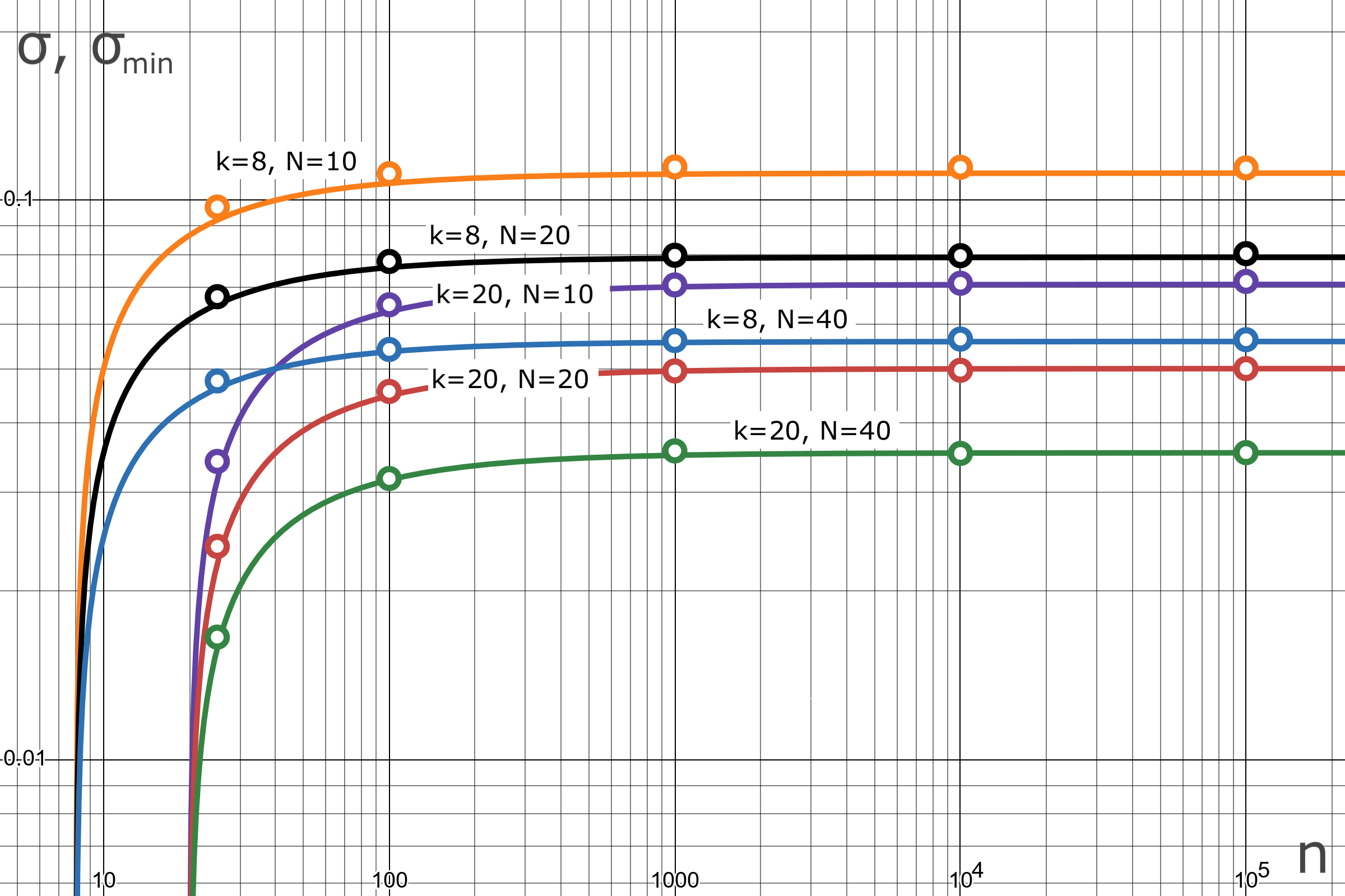Figure 1: Standard deviation of MLE estimate in comparison with the theoretical lower bound.

The solid curves in Figure 1 show the theoretical lower bounds for standard deviation $\sigma_{min}$. They are plotted according to (6) as a function of network size. The simulation results, related to the sample deviation $\sigma$, are shown as points for fixed network sizes. The results prove the efficiency of the MLE estimate. For the worst case ($k=8, N=10, n=25$), the MLE deviation (10%) differs by less than 1% from the lower bound. At increasing $k$ and $N$, the estimate precision and lower bound are practically indistinguishable. For combination ($k=20, N=40, n=25$) the MLE deviation (1.7%) differs by less than 0.01% from the lower bound.

7. Conclusion

The optimal MLE estimator differs from the estimator obtained in [2] by two significant aspects:

1. Only the maximal distances (i.e., statistics of order $k$) are used from results of $N$ $k$-lookups (sets of nodes closest to random targets). The statistics up to $k$ are irrelevant to the estimate. We can observe the minimax principle here.
2. The logarithms of normalised distances $\ln (1-u_i$) (not the distances $u_i$ directly) are used in the calculation of the sample mean to get the grouped observation.

In practice, when network size $n$ is larger than $k$, the normalised variance of efficient MLE is mainly determined by the values $N$ and $k$ (inversely proportional to), rather than $n$. The maximum of the CRLB is reached at big $n$, i.e., the minimax principle is observed again.

The results of statistical simulation prove the efficiency of the MLE estimate. For $k=8, 20$, $N \ge 10$ and $n > 100$, the variance of the MLE and the theoretical lower bound are practically indistinguishable.

8. Appendix. Joint PDF of the first k order statistics from a sample of size n

We derive formula (1) for the joint PDF of the first $k$ order statistics, $U_{(1)}, U_{(2)}, \dots, U_{(k)}$, from a random sample $U_1, U_2, \dots, U_n$ of size $n$ drawn from a standard uniform distribution on the interval $(0, 1)$.

We aim to find the probability $P(u_{1}<U_{(1)}<u_{1}+du_{1},\dots ,u_{k}<U_{(k)}<u_{k}+du_{k})$ for infinitesimal intervals. This event occurs if one sample falls into each of the $k$ intervals $(u_{i},u_{i}+du_{i})$, and the remaining $n-k$ samples are greater than $u_{k}$.

The $n$ samples must be distributed into $k+1$ categories: $k$ specific small intervals and one large interval $(u_{k},1)$. The number of distinct ways to arrange the samples into these categories is given by the multinomial coefficient:

$$\binom{n}{1, \dots ,1, n-k} = \frac {n!} {1! \dots 1!(n-k)!} = \frac {n!} {(n-k)!}$$

Let $f(u)=1$, for $u\in (0,1)$ is the standard uniform PDF. Then the probability of a single observation falling into an interval $(u_{i},u_{i}+du_{i})$ is $f(u_{i})du_{i}=1\cdot du_{i}$. The probability of an observation falling into the interval $(u_{k},1)$ is $\int _{u_{k}}^{1}f(u)du=1-u_{k}$. So, the probability for one specific arrangement is the product of these probabilities:

$$du_{1} \cdot du_{2} \dots du_{k} \cdot (1-u_{k})^{n-k}$$

The joint probability is the total number of arrangements multiplied by the probability of a single arrangement. The joint PDF is the coefficient of the volume element $du_{1}\dots du_{k}$:

$$\begin{gather*} f_{U_{(1)}, \dots, U_{(k)}}(u_1, \dots, u_k) = \frac{n!}{(n-k)!} (1 - u_k)^{n-k}, \\ \text{for} \quad 0 < u_1 < \dots < u_k < 1 \end{gather*}$$

9. References

1. Petar Maymounkov, David Mazières. Kademlia: A Peer-to-Peer Information System Based on the XOR Metric. 🔗

2. Eli Sohl. A New Method for Estimating P2P Network Size. 🔗

3. Wikipedia. Method of moments (statistics). 🔗

4. Wikipedia. Maximum likelihood estimation. 🔗

5. Wikipedia. Cramér–Rao bound. 🔗

6. Wikipedia. Order statistic. 🔗

7. Wikipedia. Trigamma function. 🔗

8. Iurii Kyrylenko. Statistical simulation of the MLE estimator for Kademlia network size. 🔗